SVM

Kernel SVM

Theory

The kernel trick allows SVMs to efficiently learn non-linear decision boundaries by implicitly mapping data to higher-dimensional spaces. Common kernels include linear, polynomial, RBF (Gaussian), and sigmoid.

Visualization

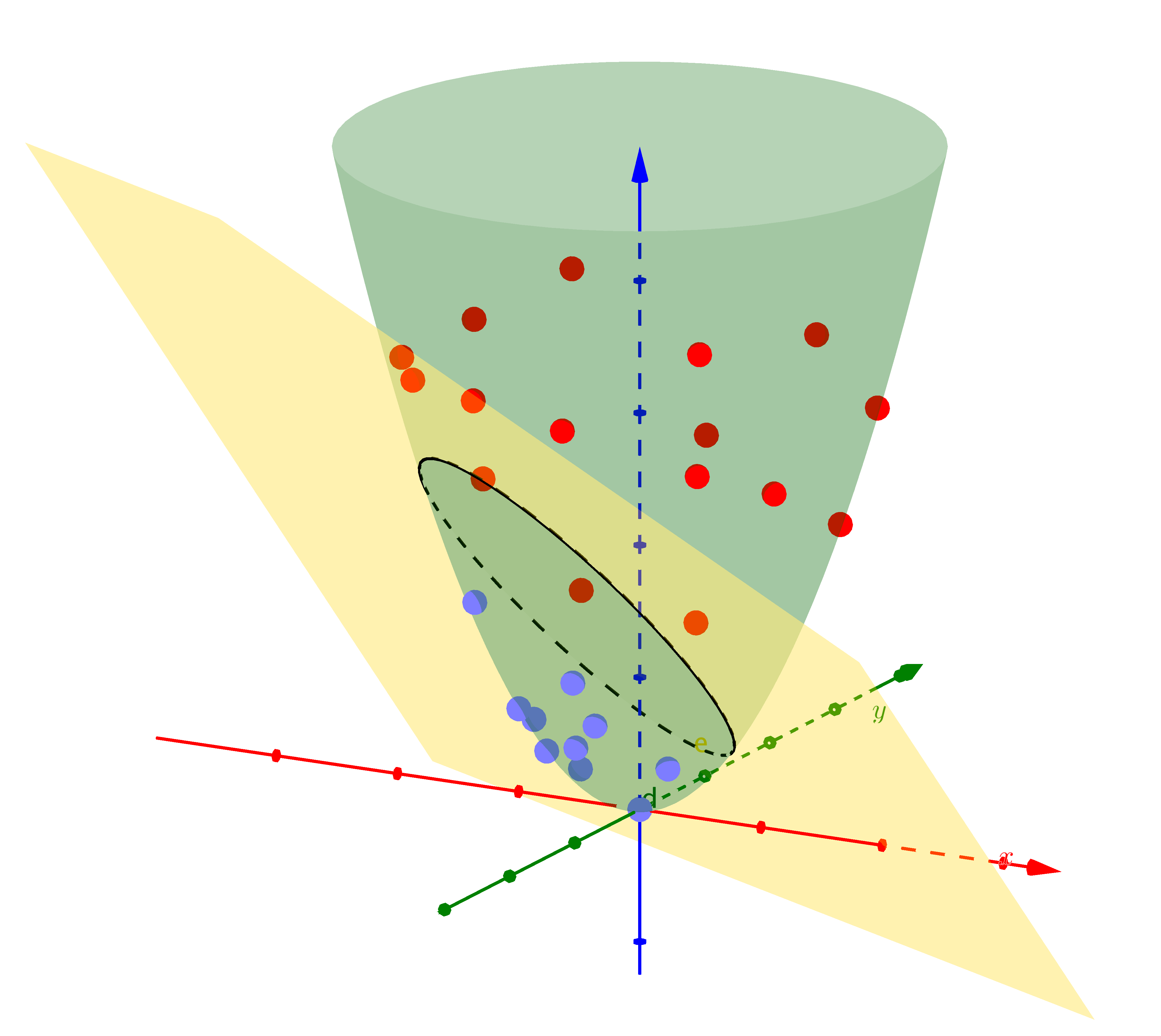
Mathematical Formulation

Kernel Function:
K(x, x') = φ(x)·φ(x')

Common Kernels:
• Linear: K(x,x') = x·x'
• Polynomial: K(x,x') = (γx·x' + r)ᵈ
• RBF: K(x,x') = exp(-γ||x-x'||²)
• Sigmoid: K(x,x') = tanh(γx·x' + r)

RBF can represent infinite dimensions!

Code Example

from sklearn import svm
from sklearn.datasets import make_moons, make_circles
import numpy as np

# Generate non-linear data
X, y = make_circles(n_samples=200, noise=0.1, 
                    factor=0.5, random_state=42)
y = np.where(y == 0, -1, 1)

# Try different kernels
kernels = ['linear', 'poly', 'rbf']

for kernel in kernels:
    if kernel == 'poly':
        clf = svm.SVC(kernel=kernel, degree=3, C=1)
    elif kernel == 'rbf':
        clf = svm.SVC(kernel=kernel, gamma='auto', C=1)
    else:
        clf = svm.SVC(kernel=kernel, C=1)
    
    clf.fit(X, y)
    accuracy = clf.score(X, y)
    
    print(f"{kernel.upper()} kernel: Accuracy={accuracy:.3f}")

# RBF with different gamma
print("\nRBF kernel with different gamma:")
for gamma in [0.1, 1, 10]:
    clf = svm.SVC(kernel='rbf', gamma=gamma, C=1)
    clf.fit(X, y)
    print(f"gamma={gamma:4.1f}: Accuracy={clf.score(X, y):.3f}")

Soft Margin SVM

Multi-class SVM