25
Dimensionality Reduction
Principal Component Analysis (1/2)
Theory
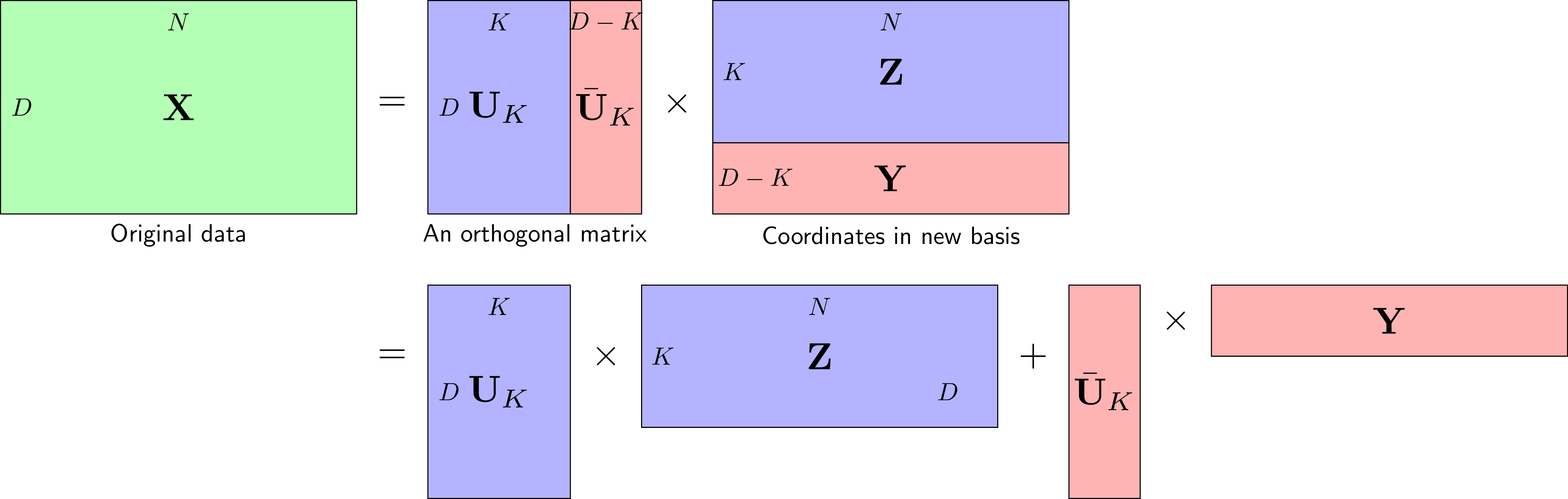
PCA is a dimensionality reduction technique that transforms data into a new coordinate system where the greatest variance lies on the first coordinate (first principal component). It's unsupervised and finds directions of maximum variance.
Visualization
Mathematical Formulation
Algorithm:
1. Standardize data (mean=0, variance=1)
2. Compute covariance matrix C = XᵀX/(n-1)
3. Compute eigenvectors and eigenvalues of C
4. Sort eigenvectors by eigenvalues (descending)
5. Project data onto top k eigenvectors

Key Properties:
• PCs are orthogonal
• First PC captures most variance
• Equivalent to SVD on centered data
Code Example
import numpy as np
from sklearn.decomposition import PCA
from sklearn.preprocessing import StandardScaler

# Generate 3D data
np.random.seed(42)
mean = [0, 0, 0]
cov = [[3, 2, 1], [2, 4, 1], [1, 1, 1]]
X = np.random.multivariate_normal(mean, cov, 200)

print(f"Original data shape: {X.shape}")
print(f"Mean: {X.mean(axis=0)}")

# Standardize
scaler = StandardScaler()
X_scaled = scaler.fit_transform(X)

# Apply PCA
pca = PCA(n_components=2)
X_pca = pca.fit_transform(X_scaled)

print(f"\nPCA transformed shape: {X_pca.shape}")
print(f"Explained variance ratio: {pca.explained_variance_ratio_}")
print(f"Cumulative variance: {np.cumsum(pca.explained_variance_ratio_)}")

# Reconstruction
X_reconstructed = pca.inverse_transform(X_pca)
reconstruction_error = np.mean((X_scaled - X_reconstructed) ** 2)
print(f"\nReconstruction MSE: {reconstruction_error:.6f}")

# Scree plot data
pca_full = PCA()
pca_full.fit(X_scaled)
print(f"\nAll explained variance ratios:")
print(pca_full.explained_variance_ratio_)